Bot or Not: Identifying Twitter Bots With Machine Learning

I recently happened across this Tweet from Mike Kearney about his new R package called botornot. It’s core function is to classify Twitter profiles into two categories: “bot” or “not”.

Having seen the tweet, I couldn’t not take the package for a spin. In this post we’ll use try to determine which of the Buffer team’s Twitter accounts are most bot-like. We’ll also test the botornot model on accounts that we know to be bots.

Data Collection

The botornot function requires a list of Twitter account handles. To gather the Buffer team’s accounts, we can collect recent tweets from the Buffer team Twitter list using the rtweet package, and extract the screen_name field from the collected tweets. First we need to load the libraries we’ll need for the analysis.

# load libraries
library(rtweet)
library(dplyr)
library(botornot)
library(openssl)
library(ggplot2)
library(hrbrthemes)
library(scales)

This query only returns tweet data from the past 6-9 days.

# gather tweets
tweets <- search_tweets("list:buffer/the-buffer-team", n = 10000)

We can gather and list the account names from the tweets dataframe.

# gather usernames
users <- unique(tweets$screen_name)
users

##  [1] "julheimer"       "julietchen"      "alfred_lua"     
##  [4] "Mike_Eck"        "Maxberthelot"    "davechapman"    
##  [7] "Kalendium"       "thedarcypeters"  "eric_khun"      
## [10] "moreofmorris"    "Brian_G_Peters"  "hitherejoe"     
## [13] "kiriappeee"      "stephe_lee"      "karamcnair"     
## [16] "hjharnis"        "Semakaweezay"    "juliabreathes"  
## [19] "joelgascoigne"   "RoyOlende"       "hailleymari"    
## [22] "ay8s"            "Bonnie_Hugs"     "kellybakes"     
## [25] "emplums"         "hamstu"          "A_Farmer"       
## [28] "tiggreen"        "kevanlee"        "mwermuth"       
## [31] "danmulc1"        "katie_womers"    "suprasannam"    
## [34] "TTGonda"         "bufferreply"     "JordanMorgan10" 
## [37] "bufferdevs"      "Ashread_"        "stevenc81"      
## [40] "KarinnaBriseno"  "bufferlove"      "no_good3r"      
## [43] "redman"          "courtneyseiter"  "goku2"          
## [46] "josemdev"        "twanlass"        "FedericoWeber"  
## [49] "CaroKopp"        "parmly"          "natemhanson"    
## [52] "michael_erasmus" "hannah_voice"    "ariellemargot"  
## [55] "djfarrelly"      "toddba"          "jntrry"         
## [58] "nystroms"        "BorisTroja"      "nmillerbooks"   
## [61] "mickmahady"      "ivanazuber"      "_pioul"         
## [64] "OCallaghanDavid"

Great, most of the team is present in this list. Interestingly, accounts like @bufferdevs and @bufferlove are also included. It will be interesting to see if they are assigned high probabilities of being bots!

The Anti Turing Test

Let’s see if the humans can convince an algorithm that they are not bots. Before we begin, it may be useful to explain how the model actually works.

According to the package’s README, the default gradient boosted model uses both users-level (bio, location, number of followers and friends, etc.) and tweets-level (number of hashtags, mentions, capital letters, etc. in a user’s most recent 100 tweets) data to estimate the probability that users are bots.

Looking at the package’s code, we can see that the model’s features also include the number of tweets sent from different clients (iphone, web, android, IFTTT, etc.), whether the profile is verified, the tweets-to-follower ratio, the number of years that the account has been on Twitter, and a few other interesting characteristics.

I’ll obfuscate the Twitter handles for privacy’s sake, but they can easily be found by reproducing the steps in this analysis or by using a MD5 reverse lookup.

The following code calculates the bot-probabilities for the Buffer team’s accounts and sorts them from most to least bot-like.

# get bot probability estimates
data <- botornot(users)

# hash the usernames
data$user_hash <- md5(data$user)

# arrange by prob ests
data %>% 
  arrange(desc(prob_bot)) %>% 
  select(-user)

## # A tibble: 64 x 2
##    prob_bot user_hash                       
##       <dbl> <chr>                           
##  1    0.999 3ff40b69a60e6210f3cbda8db1cb4ae2
##  2    0.989 3e921417f41b66f1c24862710537f192
##  3    0.985 d093563010eedd85801769f91909265d
##  4    0.964 712a4384e6681bd521c5266e16789c29
##  5    0.906 0edb7ec9098076761bd14c9c3ca97bd3
##  6    0.899 6ed84e511f386eb4942cfab089b02602
##  7    0.897 db82005412c13e740c03860b29aec7b7
##  8    0.894 8dc5886d5c56e75b89ab191e0e5958cd
##  9    0.891 a1d8e95101f88a8d7ef65d5106b7183c
## 10    0.868 fa3d30c0919008e2ab8b5e87192a13ac
## # ... with 54 more rows

The model assigns surprisingly high probabilities to many of us. The account @bufferlove is assigned a 99.9% probability of being a bot – the @bufferdevs and @bufferreply accounts are also given probabilities of 90% or higher. Verified accounts and accounts with many followers seem less likely to be bots.

Working for a company like Buffer, I can understand why this model might assign a higher-than-average probability of being a bot. We tend to share many articles, use hashtags, and retweet a lot. I suspect that scheduling link posts with Buffer greatly increases the probability of being classified as a bot by this model. Even so, these probabilities seem to be a bit too high for accounts that I know not to be bots. ?

Let’s gather more data and investigate further. We have tweet-level data in the tweets dataframe – let’s gather user-level data now. We’ll do this with the search_users function. We’ll search for users with “@buffer” in their bio and save it in the users dataframe.

# search for users
users <- search_users("@buffer")

Once we have the user list, we can join users to the data dataframe on the screen_name field.

# join dataframes
buffer_users <- data %>% 
  left_join(users, by = c("user" = "screen_name"))

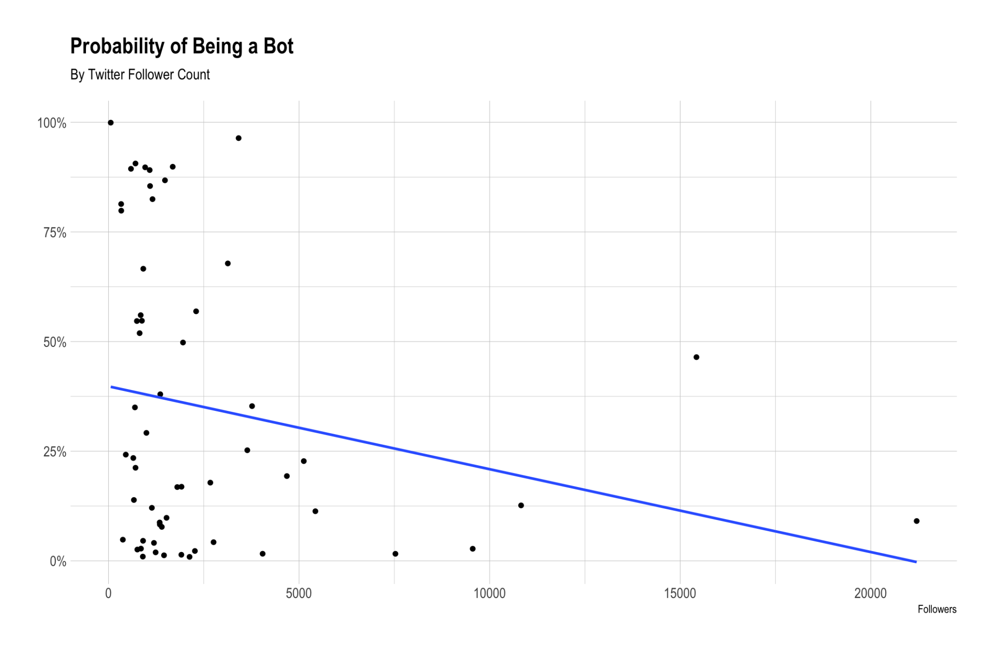
Let’s see how the probability of being a bot correlates with the number of followers that people have. We’ll leave our CEO, Joel (@joelgascoigne), out of this since he is such an outlier. He’s too famous!

We can see that there is a negative correlation between follower count and bot probability. This makes sense – bots seem less likely to have lots of followers.

Now let’s look at the relationship between bot-probability and the percentage of Tweets sent with Buffer. First we’ll calculate the proportion of tweets that were sent with Buffer for each user.

# get Buffered tweets for each user
by_user <- tweets %>% 
  mutate(sent_with_buffer = source == "Buffer") %>% 
  group_by(screen_name, sent_with_buffer) %>% 
  summarise(buffered_tweets = n_distinct(status_id)) %>%
  mutate(total_tweets = sum(buffered_tweets), 
         percent_buffered = buffered_tweets / sum(buffered_tweets)) %>% 
  filter(sent_with_buffer == TRUE) %>% 
  select(-sent_with_buffer)

# join to buffer_users dataframe
buffer_users <- buffer_users %>% 
  left_join(by_user, by = c('user' = 'screen_name'))

# replace NAs with 0
buffer_users$buffered_tweets[is.na(buffer_users$buffered_tweets)] <- 0
buffer_users$percent_buffered[is.na(buffer_users$percent_buffered)] <- 0

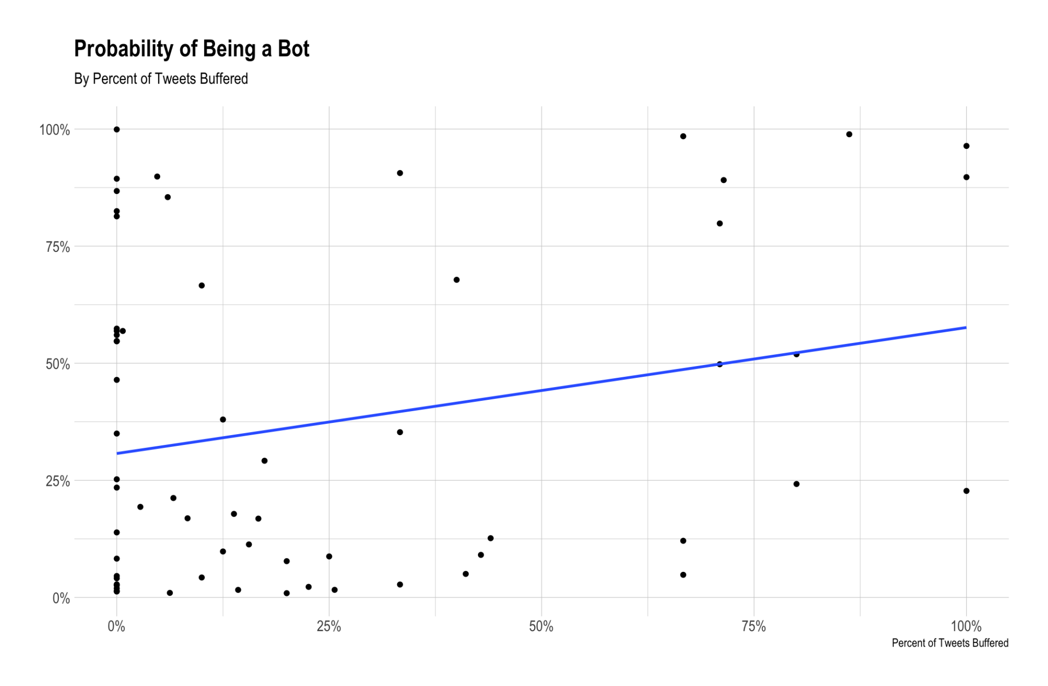
The plot below shows the relationship between the probability of being a bot and the percentage of tweets Buffered.

We can see that there is a positive correlation between the proportion of tweets Buffered and the probability of being a bot. This is interesting, but not totally unexpected.

Definitely Bots

Now it’s time to see how the model does with accounts we know to be bots. I gathered some names from this site, which maintains a few lists of Twitter bots.

# list bot accounts
bots <- c('tiny_raindrops_', 'KAFFEE_REMINDER', 'MYPRESIDENTIS', 'COLORISEBOT', 'OSSPBOT',
            'GITWISHES', 'SAYSTHEKREMLIN', 'NLPROVERBS', 'THEDOOMCLOCK', 'DAILYGLACIER')

# get botornot estimates
bot_data <- botornot(bots)

# view prob ests
bot_data %>% arrange(desc(prob_bot))

## # A tibble: 10 x 2
##    user            prob_bot
##    <chr>              <dbl>
##  1 tiny_raindrops_    1.000
##  2 thedoomclock       0.998
##  3 GitWishes          0.998
##  4 MyPresidentIs      0.998
##  5 kaffee_reminder    0.996
##  6 osspbot            0.994
##  7 saysthekremlin     0.987
##  8 NlProverbs         0.983
##  9 colorisebot        0.966
## 10 dailyglacier       0.872

Surprise! They all have been assigned very high probabilities of being bots, because they are bots. The “tiny_raindrops_” account is 100% a bot.

Conclusions

We had a fun time playing with this package – thanks for following along! I could imagine something like this being used as a weighted input in a spam prediction model in the future, however the botornot model is imperfect as-is. We’ll continue to have some fun with it and will have to consider making some tweaks before putting it into production.

Thanks for reading! Let me know if you have any thoughts or questions in the comments below!